Image segmentation based on Markov random field is a statistic-based image segmentation algorithm
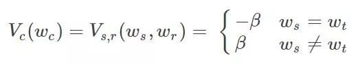
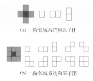
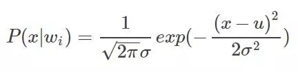
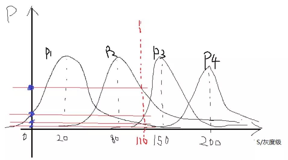
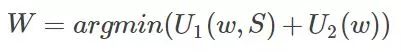
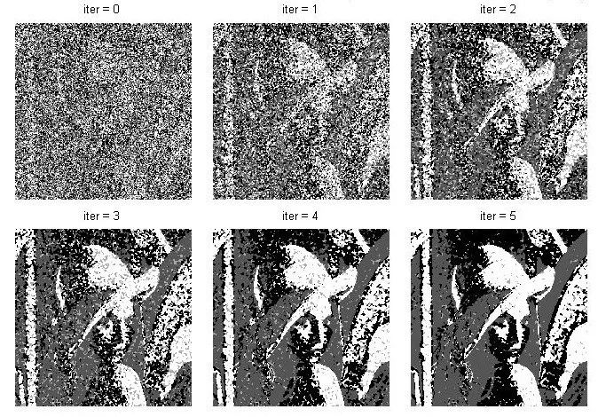
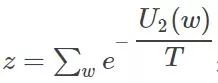
This section mainly introduces Markov's random field model and its segmentation algorithm for images. Markov-based random field (MRF) image segmentation is a statistic-based image segmentation algorithm. It has few model parameters, strong spatial constraints, and extensive use. First of all, to understand the Markov model, a pure Markov model means that the current state of a thing is related only to its previous one or n states, and it has nothing to do with the previous state. For example, today's weather is only good or bad. It was related to the weather yesterday, and it had nothing to do with the day before or even the day before yesterday. Things that meet such a characteristic are considered Markovian. Then it is extended to the image field, that is, the characteristics of a certain point in the image (usually pixel gray, color value, etc.) are only related to a small area in the vicinity, and have nothing to do with other fields. This is also true when you think about it. Most of the time, a certain pixel in the image is related to a nearby pixel. The pixel in the nearby field is black, and 80% of it is also black and well understood. One of the major uses of Markov Random Field in the image field is the segmentation of images. This paper also mainly introduces the method of image segmentation. On the image segmentation problem, from the perspective of clustering, it is a clustering problem of an image, and pixels having the same properties are set as a class. The detailed point is a label classification problem. For example, if an image is divided into four categories, then each pixel must belong to one of the four categories. Assume that the four categories are 1, 2, 3, and 4 Splitting is to find a tag class for each pixel. Well, suppose our image to be divided is S, size m*n, then put each pixel point into the set S, the image is: S=S1, S2,... Sm*n Weigh the image to be divided For the observed image. Assuming now that the segmentation is good, each pixel is divided into classes, then the final segmentation result is called W, then apparently the size of w is as large as S, W = W1, W2,...Wm*n, where all The value of w is between 1 and L. L is the maximum number of categories. For example, if L=4 above, then each w is between 1-4. This is the assumption that we know the final segmentation result W, but W is not known at the beginning? The question now is how to seek W. All we know is the observed image S. That is to say, if we know the S condition, we will find W. The probability is that the P(W|S) problem is obtained by finding P(W|S). The maximum value of the probability, that is to say according to S we calculate what the most likely segmentation tag of this image is. Based on this, the problem has only just begun. We know by Bayesian theory Observe this formula first and then look for it. Let's give some definitions first. Since W is the classification label we require, we call P(W) the prior probability of marking the field w (requiring it, without knowing in advance, it is called the prior probability, do not know if this is the case). P(S|W) is the conditional probability distribution (also called the likelihood function) of the observed value S. Look at the structure to know that this is the probability of the true pixel s in the case of the known pixel marker w. So it is a likelihood function that represents the degree to which my observation pixel and real classification situation do not look like. What is P(S)? S is the observed image. Before it is split, it's already set. I'm going to split the image. Is there any probability? No, so P(S) considers it a fixed value. Now the maximum value of P(W|S) is required, that is, the maximum value of P(S|W)P(W) is required. Let us first discuss the prior probability of P(W), the marking field w. Then we implement each pixel of the image, that is to say the probability of this pixel is the label L, some people may say, before the segmentation of the image classification label do not know, what is a certain class of label L Probability, this problem is a little bit of a bad comprehension. I think this is an egg issue. Is it chicken or egg first? We ask this chicken, but what if we don't have any eggs? A simple way is to get an egg out of the box. If he has eggs or chickens (or ducks), he can have them. Although this chicken is not like a chicken, for example, a pheasant, then there is a pheasant. The pheasant then evolved a bit, and then the next egg, the egg grew out of the pheasant 1, the pheasant 1 slightly evolved, and then the next egg, became a pheasant 2, so repeated, knowing the pheasant n, Then, when I suddenly look back and find out that the pheasant number is so similar to the chicken we wanted, then it is considered to be the chicken we want. Still not confused? In fact, many problems in the optimization clustering are egg problems. For example, the FCM algorithm once introduced, there is a question of whether egg is first given to u or first given to c. The calculation of u needs the calculation of c and c. There is a need for u. Then what to do? Assume one. Another example is the iterative process of the EM algorithm can also be seen as an egg problem, with the E step M step, back to the E step, in the M step. . . . Finally get the optimal solution. Well, back to our question, what are our problems? The probability that a pixel is a label L, start label is not, ok assuming a bar, a not, then at the beginning we initialize the entire image with a split label, although this label is wrong (pheasant), you can also assume a slightly better The tags (such as getting a pre-segmented tag with other sorting algorithms (kmeans)) (this time considered to be a pheasant number 100) (the advantage is that the algorithm can be stopped without iterating so many times at this point). Well, with the initial tag, then the probability that a pixel is the label L is determined. From this time on, we need Markov assistance. We want to ask that a pixel is the probability of the label L. At this time, the area near this pixel has also been labeled. Although this pixel also has a label, but this label is the label of the previous generation, then it goes to the next generation. It is necessary to evolve. The Markov nature tells us that the classification of this pixel is only related to the classification of some areas in the vicinity, and it has nothing to do with other fields, which means that we can decide according to the classification of the nearby areas of this pixel. What kind of pixel this pixel belongs to in the next generation? Ok, since we think that the classification of each pixel is in accordance with the Markov stochastic model, other scholars have proved that this Markov random field can be equivalent to a Gibbs random field (this is the Hammcrslcy-Clifford theorem, others prove that Then call it like this). The Gibbs random field also has a probability density function, so that instead of P(W), we use the probability P of the Gibbs random field for the image. So how does Gibbs' random probability P express? as follows: among them: , is a normalization constant, and the parameter T can control the shape of P(w), and the larger the T, the flatter. and B is the coupling coefficient, usually 0.5-1. It is not easy to be confused, not confused, so many relations, Gibbs is not easy, not finished, then what is a potential group, to put it plainly is to form a small area with this pixel connectivity testing performance, a picture is as follows: At the end of the day, at first glance, it is really complicated and incomprehensible. In fact, it is still understandable. To put it plainly, it is to check the similarity between this point and the surrounding area. Those trend groups are the objects of comparison. For example, taking a first-order potential group as an example, suppose the classification label of a certain point and its 8 fields in the vicinity after an iteration is as follows (assuming there are four types of situations): Now we need to calculate the center of the pixel in the next iteration it belongs to the first category (this generation is the third category), ok using the first-order potential energy, here need to explain that this pixel is nothing more than a category between 1-4, Then we need to calculate the next generation when it is the first, second, third and fourth groups. First assume that this point is the first category, first compare the left and right, found that all are 1-1, ok to remember B, in and B, and under, not the same, then take a look at -B, if you come to the trend group, oblique Above, 1-2, not the same as -B, obliquely below, 1-1 like B, an analogy, you can calculate the central point if it is the first type of potential group. Then if the calculation center point is the second category, it is found that the other three are not the same except that the three diagonal directions are the same. The computational assumptions are the third category and the fourth category. In this way, with each group of potential groups, the probability can be calculated. According to the formula, the band can be brought back. Finally, the probability that this point belongs to the first class, the probability of the second class, the probability of the third class, and the fourth The probability of the class, these four values ​​will be used together later to determine which class this point belongs to. You may say that you know the four probabilities and see which of the biggest ones does not come out? Note that this is only the prior probability of the first term, and the likelihood of the likelihood function is not calculated. You will see that the likelihood of this likelihood function also has four probabilities for each pixel. After the probabilities are calculated, then the probability that this point belongs to the first category is multiplied by the probabilities that both belong to the first category, and the second category is also the same. Finally, the maximum of the four probabilities is compared as the label to be labeled. . Looking at Gibbs, it is actually the degree of inconsistency between the pixel and the surrounding pixels, or the pixel around the pixel, to see how large the probability of each tag is, that is, the probability that this point belongs to the corresponding tag. Therefore, in actual programming, I did not see a few people actually using its original formula to program, but instead simplified the calculations to see how many times the labels appeared and so on. There is so much about P(W). Let's talk about P(S|W). P(S|W), a known classification label, then its pixel value (grayscale) is the probability of s. Now suppose that w=1, and the gray value of a certain pixel is s, then the expression means the probability that the pixel grayscale is s in the first class. Because the classification tags mentioned earlier, each iteration has a classification tag (although not the last tag), then we can pick out all the points that belong to the first class, considering that each point is independent , And think that all points in each class obey a Gaussian distribution (normal distribution), then in each class we can establish a Gaussian density function belonging to this class according to these points in this class, then Another pixel value, bring it to this kind of inner density function can get this probability. Similarly for the 2, 3, and 4 classes, each class can establish a Gaussian density function, so that there are four Gaussian density functions, then the probability that each point belongs to these four classes can be brought to these four Gaussians, respectively. The density function is calculated. The general form of the Gaussian density function is: As an example, suppose we now get the four Gaussian functions whose images are as follows: A certain point of gray is s = 1010, then it corresponds to P (s | W1), P (s | W2), P (s | W3), P (s | W3), respectively, as shown in the figure above Obviously, one can see that 110 has the highest probability of being in the third category, and several other probabilities can come out. Now this part also has four probabilities for each point. Combining the four probabilities for each point above, for each point, the probabilities belonging to each class are multiplied to obtain the probability that each point belongs to four classes. . This time, you can pick the biggest one of them. In this iteration, the classes that all the points belong to are updated again. Then the new class label is used as the class label for the next iteration. Repeatedly, the conditions for ending the program can be set the number of iterations, or the observation class center is not changed. . Well, the above probabilities are multiplied by the original algorithm. In fact, we can see that this calculation consists of two parts. In general, we say that each part of these two parts forms an energy. In other words, the energy function is optimized. It can be expressed as follows: Multiply the probabilities like above to take the logarithms in practice and add them up. A deeper Markov random field can go to the relevant papers. Although the method may not be the same, the principle is the same. The following uses Conditional Iteration Algorithm (ICM) to illustrate the application of MRF in image segmentation. The programming platform is matlab. The related code is as follows: Clc Clear Close all Img = double(imread('lena.jpg'));%more quickly Cluster_num = 4;% Set the number of categories Maxiter = 60;% maximum number of iterations %------------- Initialize Tags Randomly ---------------- Label = randi([1,cluster_num],size(img)); %-----------kmeans initializes pre-segmentation ---------- % label = kmeans(img(:),cluster_num); % label = reshape(label,size(img)); Iter = 0; while iter maxiter %-------Calculate Prior Probability --------------- % Here I use the same pixel and 3*3 tags % or not as calculated probability %------ Collect up and down, left, right, and other eight directions of labels -------- Label_u = imfilter(label,[0,1,0;0,0,0;0,0,0],'replicate'); Label_d = imfilter(label,[0,0,0;0,0,0;0,1,0],'replicate'); Label_l = imfilter(label,[0,0,0;1,0,0;0,0,0],'replicate'); Label_r = imfilter(label,[0,0,0;0,0,1;0,0,0],'replicate'); Label_ul = imfilter(label,[1,0,0;0,0,0;0,0,0],'replicate'); Label_ur = imfilter(label,[0,0,1;0,0,0;0,0,0],'replicate'); Label_dl = imfilter(label,[0,0,0;0,0,0;1,0,0],'replicate'); Label_dr = imfilter(label,[0,0,0;0,0,0;0,0,1],'replicate'); P_c = zeros(4,size(label,1)*size(label,2)); % Calculates the same number of pixels 8 field labels relative to each class for i = 1: cluster_num Label_i = i * ones(size(label)); Temp = ~(label_i - label_u) + ~(label_i - label_d) + . . . ~(label_i - label_l) + ~(label_i - label_r) + . . . ~(label_i - label_ul) + ~(label_i - label_ur) + . . . ~(label_i - label_dl) +~(label_i - label_dr); P_c(i,:) = temp(:)/8;% calculation probability End P_c(find(p_c == 0)) = 0.001;% prevents the occurrence of 0%--------------- calculation of the likelihood function ------------- --- Mu = zeros(1,4); Sigma = zeros(1,4); % finds the Gaussian parameters for each class - the mean variance for i = 1: cluster_num Index = find(label == i);% Find each class point Data_c = img(index); Mu(i) = mean(data_c); %-mean Sigma(i) = var(data_c); % Variance End P_sc = zeros(4,size(label,1)*size(label,2)); % for i = 1: size(img,1)*size(img,2) % for j = 1:cluster_num % p_sc(j,i) = 1/sqrt(2*pi*sigma(j))*. . % exp(-(img(i)-mu(j))^2/2/sigma(j)); % end % end %------ Calculate the likelihood probability of each pixel belonging to each class -------- %------ In order to speed up the operation, the loop is changed to a matrix operation --------for j = 1:cluster_num MU = repmat(mu(j),size(img,1)*size(img,2),1); P_sc(j,:) = 1/sqrt(2*pi*sigma(j))*. . Exp(-(img(:)-MU).^2/2/sigma(j)); End % Find the maximum probability of union with the tag, take the logarithm to prevent the value is too small [~,label] = max(log(p_c) + log(p_sc)); % changed size for easy display Label = reshape(label,size(img)); %---------show ----------------if ~mod(iter,6) Figure; n=1; End Subplot(2,3,n); Imshow(label,[]) Title(['iter = ',num2str(iter)]); Pause(0.1); n = n+1; Iter = iter + 1; End Set the number of categories to cluster_num=4 and paste a few intermediate results: In addition to the comments above, the above program is to say that for the need of pre-classification, both the random classification and the kmeans pre-classification are written in the program, and the posted results are all randomly initialized. When we go to the experiment, we can find that if we use the kmeans pre-classification, the result of the iterative starting segmentation is very good, and the program will change a little bit on this basis. The advantage of adopting the kmeans pre-classification is that the segmentation result will reach stability more quickly. And more accurate. The use of random pre-classification, the results of the segmentation can also be considered, this method is a local optimal solution, of course, kmeans also get a local optimal solution (dare not say the optimal solution), but the previous local The optimal solution is worse than the local optimal solution after kmeans, especially when the number of segmentation categories is larger, the effect of kmeans pre-classification is obviously better than random pre-classification. Because the larger the number of categories is, the larger the equivalent dimension is, and the more local optimal solutions it has, the less likely it is to go from the random pre-classification (worst case) to the optimal solution. A local optimum solution can't be reached. In a sense, this segmentation is an np-hard problem, and it is difficult to find the optimal solution for segmentation. Insulated Power Cable,Bimetallic Crimp Lugs Cable,Pvc Copper Cable,Cable With Copper Tube Terminal Taixing Longyi Terminals Co.,Ltd. , https://www.txlyterminals.com


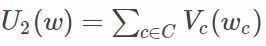 C is a collection of all potential groups.
  For potential group potential energy,